Bearing Load Calculation: From Shaft Forces to Fr, Fa and L10
Bearing Load Calculation: From Shaft Forces to Fr, Fa and L10
Every bearing selection guide starts with a table that says “determine your radial load Fr and
axial load Fa first”. Almost none of them tells you where those two numbers come from. In a
real machine they are not measured, they are not in the catalogue, and they are not the forces on
the gear or the belt. They are the reaction forces at the bearing seats, and getting
from a transmitted torque to those reactions takes a free-body diagram, two planes of static
equilibrium, and a decision about which bearing locates the shaft axially.
This article runs that whole chain on one shaft, end to end, with numbers: torque and speed
→ the three force components of a helical gear → tight-side and slack-side belt tensions
→ support reactions in the vertical and horizontal planes → vector-summed radial loads
→ axial load allocation → service factor → equivalent dynamic load P →
ISO 281 L10h → required dynamic load rating C. The load case we
arrive at is exactly the one used in our bearing type selection decision
matrix, so you can follow the arithmetic straight through to a bearing choice.
About the numbers: the geometry, forces, ratings and factors in this
worked example are illustrative magnitudes for teaching the method, not catalogue values for
any specific product. Substitute the actual dimensions, duty and catalogue ratings before making a
purchasing decision.
1. Why the load case is the part people get wrong
A bearing fails because of the load at the bearing, not the load at the gear. Between the
two there is a lever system that can amplify, redistribute or cancel forces. A pulley hung outboard
of the last support is the classic example: a 5 kN belt pull can produce a 7.7 kN reaction at one
support and almost nothing at the other, because the moment arm outside the span has to be balanced
by an opposing force inside it. If you simply “divide the total load by two”, every downstream
calculation is wrong.
Three consequences make this worth doing properly:
- Life is nonlinear. L10 scales with (C/P)p,
with p = 3 for ball bearings and 10/3 for roller bearings. A 20% error in the reaction
force becomes roughly a 45–50% error in predicted life. - The two bearings rarely carry the same load. Sizing both from an average is
simultaneously wasteful on the lightly loaded seat and unsafe on the heavily loaded one. - Axial load is not shared. In a locating/floating arrangement the axial force
goes entirely to one bearing. Splitting it 50/50 understates P at the locating bearing
and overstates it at the floating one.
The remedy is a fixed sequence. Do not open a catalogue until step 7.
2. The calculation chain at a glance
Eight steps, each with one output that becomes the next step’s input. Keep them separate: most
mistakes come from collapsing two steps into one, or applying a factor twice.
| Step | What you compute | Output | Common trap |
|---|---|---|---|
| 1 | Torque from power and speed; gear force components | Ft, Frgear, Fa | Using normal pressure angle without the helix correction |
| 2 | Belt effective pull and total radial pull on the pulley | T1, T2, Fbelt | Confusing T1−T2 with T1+T2 |
| 3 | Static equilibrium in two perpendicular planes | RAv, RBv, RAh, RBh | Forgetting the overhung moment arm |
| 4 | Vector sum of the two planes at each seat | FrA, FrB | Adding reactions arithmetically instead of geometrically |
| 5 | Axial load allocation (locating / floating) | Fa per bearing | Splitting Fa equally between supports |
| 6 | Application / shock factor and duty cycle | fd, duty-weighted load | Multiplying fd into reactions and again into P |
| 7 | Equivalent dynamic load P = fd(X·Fr + Y·Fa) | P in kN | Using X/Y from the wrong Fa/Fr band |
| 8 | L10h and required C from ISO 281 | Life in hours, Creq | Using the ball exponent for a roller bearing |
3. Build the mechanical model first
Our example is a horizontal geared drive shaft: a helical gear inside the bearing span, a V-belt
pulley overhung beyond the right-hand support, and two bearing seats. Support A is
the floating (non-locating) bearing; support B is the locating bearing and therefore
takes the shaft’s axial load. The geometry is deliberately simple so every number can be checked by
hand.
| Item | Symbol / position | Value |
|---|---|---|
| Support A (floating) | xA | 0 mm |
| Support B (locating) | xB | 300 mm |
| Helical gear centre | xG | 100 mm (inside the span) |
| Pulley centre | xP | 390 mm (90 mm overhung past B) |
| Transmitted torque | T | 687 N·m |
| Shaft speed | n | 720 rpm (51.8 kW) |
| Gear pitch diameter | dg | 200 mm |
| Gear normal pressure angle / helix angle | αn / β | 20° / 20° |
| Pulley pitch diameter | dp | 500 mm |
| Belt tension ratio | r = T1/T2 | 3.2 |
We resolve forces into two perpendicular planes. The vertical plane V carries the
gear’s separating (radial) force and the belt pull, both acting downward. The horizontal
plane H carries the gear’s tangential force. Axial force acts along the shaft and is handled
separately in step 5. Forces in the two planes never get added to each other — they get combined
as vectors at the very end.
4. Step 1 — torque, power and the three gear forces
A helical gear does not apply one force to the shaft. It applies three mutually perpendicular
components, and mixing them up is the single most common source of a wrong load case. With torque
T and gear pitch diameter dg:
| Component | Formula | Direction | In our example |
|---|---|---|---|
| Tangential (transmits the torque) | Ft = 2T / dg | Horizontal plane H | 2 × 687 / 0.200 = 6.870 kN |
| Radial / separating | Fr,gear = Ft · tanαn / cosβ | Vertical plane V | 6.870 × 0.3640 / 0.9397 = 2.661 kN |
| Axial (thrust from the helix) | Fa = Ft · tanβ | Along the shaft | 6.870 × 0.3640 = 2.500 kN |
Two details matter. First, the radial component uses the normal pressure angle divided by
cosβ; using tanαn alone understates it by about 6% at a 20° helix. Second,
the axial component exists only because the teeth are helical — a spur gear has
Fa = 0 and the whole axial-load question disappears. Reversing the direction of
rotation reverses which side of the bearing sees the thrust, but not its magnitude.
Power is a useful cross-check: T · ω = 687 × (2π × 720/60)
= 51.8 kW. If a customer quotes power and speed instead of torque, invert this first:
T = 9550 · PkW / nrpm N·m.
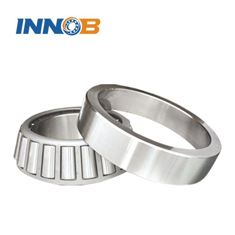
Combined-load types such as tapered roller bearings and
spherical roller bearings exist precisely because a shaft often
has to carry all three components at once; see our
tapered roller bearing selection guide for how paired arrangements
handle the axial part.
5. Step 2 — belt tension: T1−T2 is not T1+T2
Here is the step that changes the answer more than any other, and the one almost every supplier
blog omits. A belt transmits torque through the difference between tight-side tension T1 and
slack-side tension T2, but the shaft feels their sum. Both numbers are needed, and they are
not interchangeable.
Fe = T1 − T2 = T / (dp/2)
and Fbelt = T1 + T2
| Quantity | Calculation | Value |
|---|---|---|
| Effective circumferential pull Fe | 687 / 0.250 | 2.748 kN |
| Slack-side tension T2 | Fe / (r − 1) = 2.748 / 2.2 | 1.249 kN |
| Tight-side tension T1 | r × T2 = 3.2 × 1.249 | 3.997 kN |
| Radial pull on the shaft Fbelt | T1 + T2 | 5.246 kN |
Note the ratio: the shaft sees 5.246 kN of radial load while transmitting only 2.748 kN of useful
circumferential force — nearly twice as much. The excess is installed pre-tension, and it is
present even at zero torque, which is why a belt drive can brinell a bearing while idling. Over-tension
is a maintenance fault, not a design input, and step 12 quantifies exactly what it costs in life.
The same logic applies to chain drives (without the elastic tension ratio) and to any overhung
load. If the drive is a coupling instead, there is no deliberate radial pull at all, but there is
usually a residual misalignment force — measure it rather than assume zero.
6. Step 3 — static equilibrium in two planes
Now treat the shaft as a simply supported beam with two supports 300 mm apart. Work each plane
separately, using ΣF = 0 and ΣM = 0 about support A. All distances are in mm from A.
Vertical plane V — gear separating force 2.661 kN at x = 100 mm, belt pull
5.246 kN at x = 390 mm:
RAv + RBv = 2.661 + 5.246 = 7.907 kN
RBv × 300 = 2.661 × 100 + 5.246 × 390 = 2312.0 kN·mm
→ RBv = 7.707 kN, RAv = 0.200 kN
Horizontal plane H — only the gear tangential force 6.870 kN at x = 100 mm:
RBh × 300 = 6.870 × 100 = 687.0 → RBh = 2.290 kN,
RAh = 4.580 kN
| Plane | Applied loads | Reaction at A | Reaction at B |
|---|---|---|---|
| Vertical V | 2.661 kN @ 100 mm; 5.246 kN @ 390 mm | 0.200 kN | 7.707 kN |
| Horizontal H | 6.870 kN @ 100 mm | 4.580 kN | 2.290 kN |
The 390 mm term is the whole story. Because the pulley sits outside the span, its moment
about A is larger than a load inside the span would produce, and the only way to balance it is a large
upward reaction at B plus a very small reaction at A. If you wrongly used 300 mm for the pulley
position, RBv would come out at 6.133 kN instead of 7.707 — a 20% understatement of
the vertical reaction at the critical bearing. Support A’s vertical reaction is nearly zero not
because there is no load, but because the overhung load is trying to lift it.
7. Step 4 — combine the planes into the real Fr
The four reactions are components, not answers. A bearing sees the resultant of the vertical and
horizontal components at its seat:
Fr = √(Rv2 + Rh2)
| Seat | Rv | Rh | Resultant Fr | Comment |
|---|---|---|---|---|
| A (floating) | 0.200 kN | 4.580 kN | 4.58 kN | Dominated by the gear tangential force |
| B (locating) | 7.707 kN | 2.290 kN | 8.04 kN ≈ 8.0 kN | Dominated by the overhung belt pull; governs the selection |
Adding the components arithmetically at B would give 9.997 kN, a 24% overstatement; averaging all
applied loads across two supports would give 7.389 kN, an 8% understatement of the governing bearing.
Both are wrong in different directions, which is why an “about right” load case is not good enough
once the life exponent is applied.
We will size from bearing B, the heavier seat, and round to Fr = 8.0 kN. That is
the number carried into the worked selection example in our companion
guide. In practice you would also run the same arithmetic for A and check that the lighter seat still
meets minimum load and fit requirements.
8. Step 5 — who carries the axial load?
The 2.500 kN gear thrust acts along the shaft. In a locating/floating arrangement it is carried
entirely by one bearing, the locating one, and then passed into the housing. The
floating bearing is allowed to slide axially so that thermal growth does not preload the pair.
| Seat | Role | Fr | Fa | Typical type |
|---|---|---|---|---|
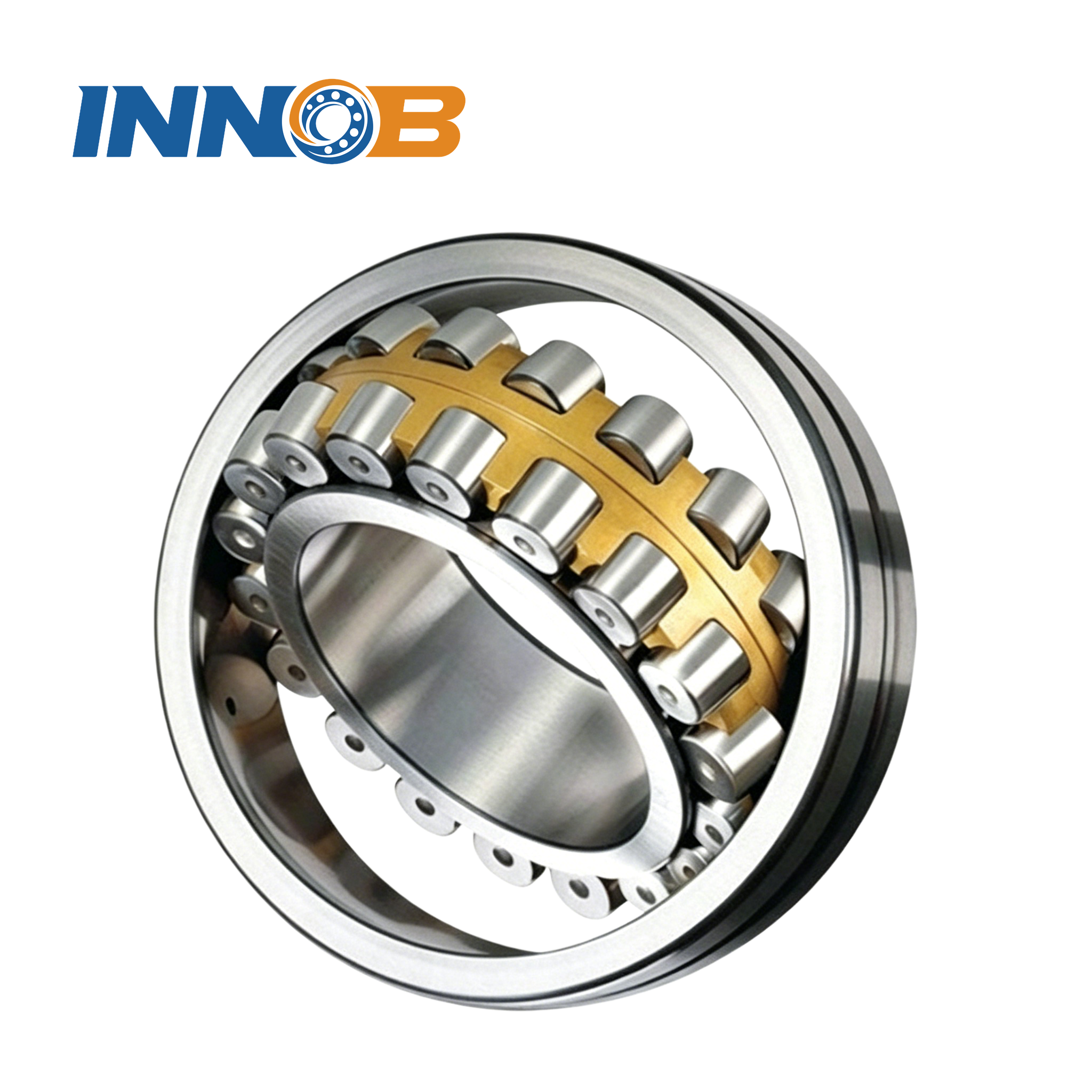
| A | Floating / non-locating | 4.58 kN | 0 kN | NU or N cylindrical roller, or a deep groove ball bearing with a sliding outer-ring fit |
| B | Locating | 8.04 kN | 2.500 kN | Spherical roller, paired tapered roller, or paired angular contact depending on alignment and stiffness |
Two exceptions are worth flagging. If both bearings are arranged as an opposed tapered-roller or
angular-contact pair, the axial load is shared through the pair’s internal load distribution and the
P calculation uses pair-specific factors — not a simple 50/50 split. If there is no
axial load at all (spur gear, no thrust), the locating bearing still needs to be defined for shaft
positioning, but Fa = 0 and the X/Y choice collapses to the pure-radial case.
Also remember that axial load changes Fa/Fr, which decides the X and Y
factors in step 7. Here Fa/Fr = 2.5 / 8.0 = 0.313. Pure axial cases — vertical shafts,
hooks, screw presses — are a different calculation entirely and use
thrust ball or thrust roller bearings; see our
thrust bearing overview.

9. Step 6 — nominal loads versus design loads
Everything so far is a static, steady-state nominal load. Real machines add shock, start-stop
cycles, and duty segments where load and speed both vary. ISO 281 handles this with an application
factor fd applied when forming P, not when solving the reactions. Applying it in
both places would double-count it: our P would be 21.31 kN instead of 16.39 kN, and the predicted
life would collapse by more than half for no physical reason.
| Operating character | Illustrative fd | Typical examples |
|---|---|---|
| Smooth, steady, no shock | 1.0 – 1.2 | Fans, light conveyors, generators |
| Moderate shock, frequent starts | 1.2 – 1.5 | Geared drives, mixers, machine tools (our example: 1.3) |
| Heavy shock, reversing | 1.5 – 2.0 | Crushers, rolling mills, excavators |
| Severe impact / very heavy | 2.0 – 3.0 | Presses, pile drivers, severe mining duty |
These bands are illustrative guidance, not a standard table; use the factors published by the
bearing manufacturer for your application class. If the machine runs a genuine duty cycle — say
40% of the time at full load and 60% at half load — the rigorous route is a cumulative damage
calculation: compute P for each segment, obtain each segment’s L10h, and
combine them with the Palmgren–Miner rule 1/L = Σ(ui/Li), where
ui is the fraction of time spent in segment i. A single “average load” is a
conservative shortcut only when the exponent is applied to the weighted cube (or 10/3 power) of the
loads, never to the loads themselves.
10. Step 7 — equivalent dynamic load P
ISO 281 reduces a combined radial and axial load to one equivalent radial load that would produce
the same fatigue life:
P = fd · (X·Fr + Y·Fa)
X and Y depend on the bearing type and on whether Fa/Fr exceeds a
limiting value e. For the governing bearing B, using the same illustrative factors as the
companion selection example (e = 0.23, X = 0.67, Y = 2.9 for a spherical
roller bearing):
- Fa/Fr = 0.313 > e = 0.23, so the axial term stays in with both factors.
- P = 1.3 × (0.67 × 8.0 + 2.9 × 2.5) = 1.3 × (5.36 + 7.25) = 1.3 × 12.61 = 16.39 kN.
The axial component contributes 7.25 kN of the 12.61 kN bracket — more than the radial
component — because Y = 2.9 penalises axial load heavily in this bearing family. This
is the step where a wrong Fa from step 5 does the most damage. Had we split the axial load
equally (1.25 kN each), P would have been only 11.96 kN and the life prediction would have been
roughly 2.6× too optimistic.
For a deep groove ball bearing, e and Y are themselves functions of
Fa/C0, so you need a trial bearing before you can finish P. The full
three-candidate comparison — deep groove ball, paired tapered roller and spherical roller,
including their X/Y values — is worked out in our
bearing type selection decision matrix; this article stops at the load
case that feeds it. Factors e, X and Y must always come from the actual
manufacturer’s catalogue, never from memory.
11. Step 8 — L10h and the capacity you actually need
ISO 281 basic rating life in million revolutions is L10 = (C/P)p,
with p = 3 for ball bearings and 10/3 for roller bearings. Converting to hours at speed
n:
L10h = (106 / 60n) · (C/P)p
At 720 rpm, 106/(60 × 720) = 23.15 h per million revolutions.
With the illustrative C = 178 kN for a 22214 spherical roller bearing, P = 16.39 kN
and p = 10/3:
L10h = 23.15 × (178 / 16.39)10/3 = 65,623 h
Rearranged for a 20,000 h target: Creq = P · (20,000 / 23.15)1/p
= 16.39 × 7.60 = 124.6 kN. The candidate with C = 178 kN clears the
target by roughly three times, which is where the companion guide takes over and checks the
constraints that are not about life — 0.4° of frame misalignment, a 150 mm outside
diameter envelope, speed and lubrication.
| Stage | Value | Where it came from |
|---|---|---|
| Torque / speed | 687 N·m / 720 rpm | Step 1 input |
| Fr / Fa at bearing B | 8.0 / 2.5 kN | Steps 1–5 |
| fd | 1.3 | Step 6 |
| P | 16.39 kN | Step 7 |
| L10h at C = 178 kN | 65,623 h | Step 8 |
| Creq for 20,000 h | 124.6 kN | Step 8, rearranged |
That chain — from a quoted torque to a required catalogue rating — is the deliverable.
If a customer changes the pulley diameter, the belt pre-tension, the gear helix angle or the support
span, every row below the change has to be recomputed; none of them can be reused on assumption.
12. Sensitivity: belt pre-tension moves life more than torque does
This is the calculation competitors never show, and the one that usually changes a maintenance
decision. Keep torque, geometry and Fa fixed, and vary only the belt tension ratio
r = T1/T2. A lower ratio means more installed pre-tension for the same transmitted torque
— the shaft never sees a newton of extra useful work, but it carries a lot more radial load.
| r = T1/T2 | Belt pull T1+T2 (kN) | RBv (kN) | FrB (kN) | P (kN) | L10h (h) |
|---|---|---|---|---|---|
| 2.0 (over-tensioned) | 8.244 | 11.604 | 11.828 | 19.73 | 35,402 |
| 2.5 | 6.412 | 9.223 | 9.503 | 17.70 | 50,799 |
| 3.2 (design case) | 5.246 | 7.707 | 8.040 | 16.43 | 65,159 |
| 4.0 | 4.580 | 6.841 | 7.214 | 15.71 | 75,649 |
| 5.0 (loose, slip risk) | 4.122 | 6.246 | 6.652 | 15.22 | 84,067 |
| No belt load (reference only) | 0 | 0.887 | 2.456 | 11.56 | 210,002 |
Going from r = 5.0 to r = 2.0 — a plausible range of how the same belt might be tensioned in
the field — cuts predicted life from 84,067 h to 35,402 h, a 58% reduction,
with no change in transmitted power. The rows use the unrounded FrB = 8.040 kN,
which is why the design-case row reads 65,159 h while the round-number chain in step 11 gives
65,623 h; the difference is 0.7% and is purely rounding.
The practical conclusions: specify a tension ratio, measure belt tension at installation and
re-check it after run-in, and never “tighten it until it stops squeaking”. If a bearing at an
overhung pulley fails early with no change in duty, the belt tension is the first thing to measure.
Lubrication and clearance matter too — see our notes on
bearing clearance and
choosing a bearing lubricant — but they cannot recover a life deficit
created by a 3 kN surplus of radial load.
13. Eight mistakes that quietly halve (or double) the answer
Each row below was computed from the same example, so the size of the error is visible. The last
column shows what the mistake does to the governing bearing’s load or life.
| Mistake | Wrong value | Correct value | Effect |
|---|---|---|---|
| Use T1+T2 as the transmitted force | 5.246 kN “circumferential” | 2.748 kN | Nearly 2× overstates torque / understates pre-tension |
| Average all applied loads over two supports | 7.389 kN each | A 4.58 / B 8.04 kN | 8% low at B, 61% high at A |
| Add the two planes arithmetically | 9.997 kN at B | 8.040 kN | 24% high; life understated by ~2× |
| Use 300 mm instead of 390 mm for the overhung pulley | RBv = 6.133 kN | 7.707 kN | 20% low on the vertical reaction |
| Split the axial load 50/50 | 1.250 kN each | 2.500 / 0 kN | P understated ~27%; life overstated ~2.6× |
| Apply fd to reactions and again to P | P = 21.31 kN | 16.39 kN | Life understated by ~55% |
| Use the ball exponent p = 3 for a roller bearing | wrong (C/P)3 | (C/P)10/3 | Life error grows with C/P |
| Assume steady full load instead of a duty cycle | one P for all hours | segment-wise P and Miner’s rule | Can overstate or understate by multiples |
Notice that the errors do not cancel: several of them push in the same direction. A load case built
from two or three shortcuts is not “approximately right”, it is simply a different machine.
14. What to measure before you calculate
The arithmetic is only as good as the inputs. This is the shortlist we ask customers for when a
load case has to be rebuilt from an existing machine rather than designed from scratch.
| Input | Why it is needed | How it is usually obtained |
|---|---|---|
| Power / torque and speed, plus duty segments | Sets Ft and L10h | Motor nameplate, drive log, or measured current |
| Gear: pitch diameter, αn, β, hand of helix | Splits torque into Ft, Fr, Fa | Gear drawing or tooth count + module |
| Pulley / sprocket diameter, overhang, belt type and tension | Dominates the reaction at the adjacent bearing | Layout drawing; tension gauge at installation |
| Distance between bearing centres and all load positions | Moment arms for ΣM = 0 | Assembly drawing |
| Which bearing locates axially; thermal growth allowance | Decides Fa allocation | Arrangement drawing; see roller bearing arrangements |
| Shock / start frequency, reversing, ambient temperature | fd, clearance class, lubrication | Operating history |
| Available envelope: bore, OD, width | Eliminates candidates after life is computed | Housing measurement |
| Existing bearing designation and failure appearance | Sanity check on the computed load direction | Photos of the failed part |
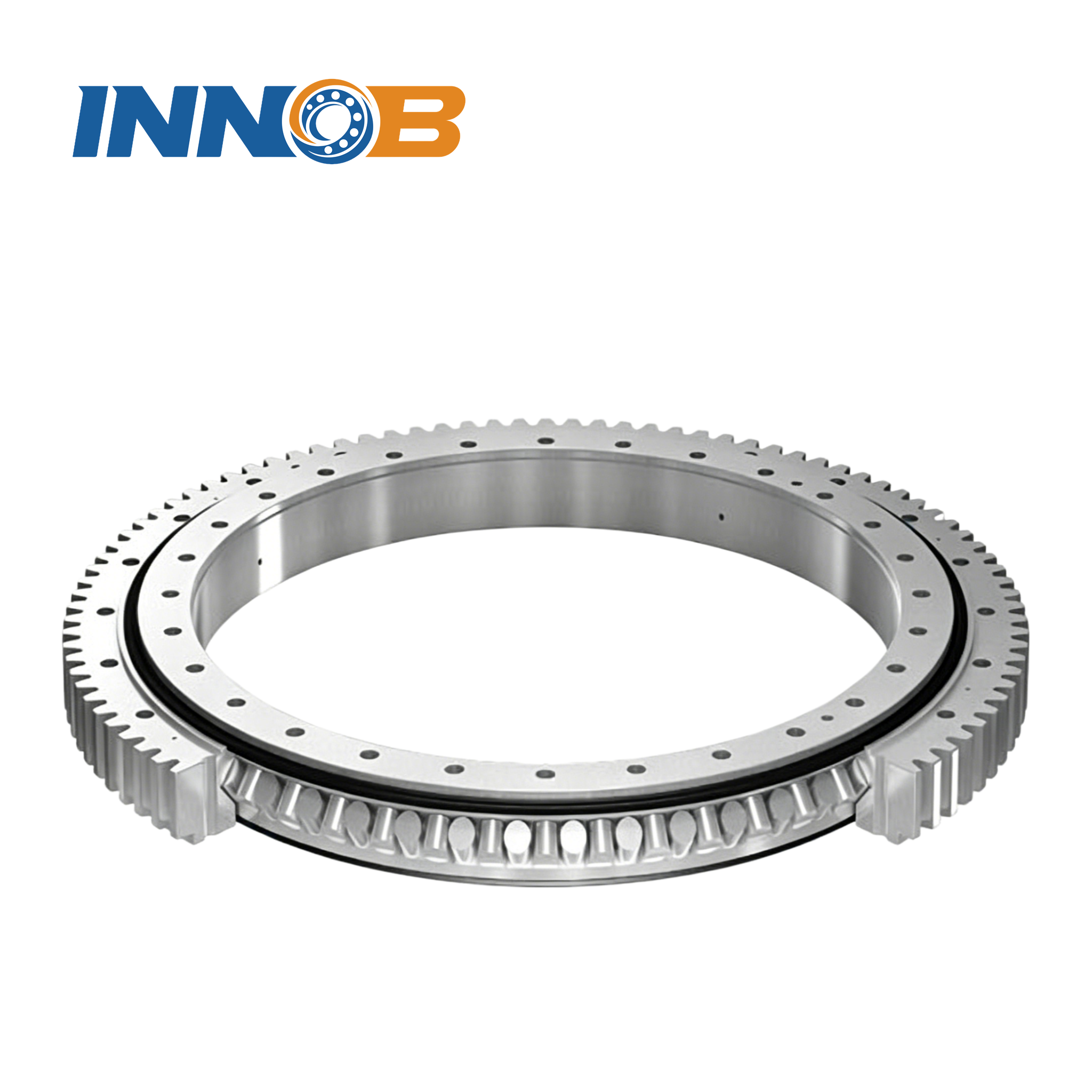
For structures that rotate slowly under a tilting moment rather than a spinning shaft, the whole
model changes: the load case is built from axial force, radial force and tilting moment at the
mounting plane, not from gear and belt reactions. Our
slewing bearing selection overview and
crossed roller vs ball slewing comparison cover that case, and the
rolling bearing vs slewing bearing boundary explains where the
two approaches diverge.
Send us the shaft layout, get the load case back
The chain above is what our engineers run before quoting a bearing: gear and belt data, support
geometry, which seat locates axially, duty cycle, target life and envelope. Give us those inputs and
we will return the computed Fr and Fa at each seat, the equivalent dynamic load
P, the resulting L10h and the shortlist of types that fit — including
what would have to change in the shaft or frame if none of them does.
Send your operating data to our engineering team.
You can also browse deep groove ball,
tapered roller,
cylindrical roller,
spherical roller,
angular contact,
thrust and
thin-section bearings for the families that appear in this load chain.
Related reading
- Bearing Type Selection: A Decision Matrix with a Worked Example — takes this exact load case (Fr 8.0 kN, Fa 2.5 kN, 720 rpm, 20,000 h) through P, L10h and three candidate bearings.
- Tapered Roller Bearing Selection Guide — paired arrangements, preload and endplay for the locating seat.
- Spherical & Cylindrical Roller Bearings — the two high-capacity roller families and where they belong in an arrangement.
- Angular Contact vs Deep Groove Ball Bearings — how the X/Y factors differ when Fa/Fr rises.
- Важность зазора в подшипниках — what fits and temperature do to the clearance you selected.
- The Types of Ball Bearings — a closer look at the ball-bearing families.
- Crossed Roller vs Ball Slewing Bearings — the decision-matrix approach applied to slewing rings.
- How to Choose the Right Slewing Bearing — the alternative load chain for slow-rotating structures.
Frequently Asked Questions
How do you calculate the radial load on a bearing?
Draw a free-body diagram of the shaft, resolve all gear, belt, chain or coupling forces into two perpendicular planes, solve static equilibrium (sum of forces and moments about one support) in each plane, then take the vector sum of the two reaction components at that bearing seat: Fr = sqrt(Rv^2 + Rh^2). The result is the reaction at the seat, not the force applied at the gear.
Is belt tension T1+T2 or T1-T2?
Both, for different purposes. T1-T2 is the effective circumferential force that transmits torque (T1-T2 = T/(d/2)). T1+T2 is the total radial pull the shaft and bearings actually carry. With a tension ratio of 3.2, a belt transmitting 2.748 kN puts 5.246 kN of radial load on the shaft.
Which bearing takes the axial load?
In a locating/floating arrangement the axial load goes entirely to the locating bearing; the floating bearing is free to move axially to accommodate thermal growth. Splitting axial load equally between the two supports understates P at the locating bearing and can overstate life by more than two times. Opposed tapered or angular contact pairs use pair-specific factors instead.
What is equivalent dynamic load P?
P is the single radial load that would give the same fatigue life as the actual combined radial and axial loading. It is P = fd*(X*Fr + Y*Fa), where X and Y depend on the bearing type and on whether Fa/Fr exceeds the limit e. Because life scales with (C/P)^p, an error in P is amplified.
How does an overhung pulley affect bearing loads?
An overhung load acts outside the bearing span, so its moment about the far support is larger than the same load inside the span. The near support reaction rises sharply while the far support reaction can approach zero or reverse. In our example a 5.246 kN belt pull at 90 mm overhang produces a 7.707 kN vertical reaction at the adjacent bearing.
Should I apply a service factor to the reaction forces?
Apply the application factor fd once, when forming the equivalent dynamic load P. Applying it to the static reactions and again to P double-counts the shock allowance and can understate life by more than half. For a real duty cycle, compute P per segment and combine lives with Miner's rule.
How do I get torque from motor power and speed?
T (N.m) = 9550 * P(kW) / n(rpm). For 51.8 kW at 720 rpm that is 687 N.m. Torque then gives the gear tangential force Ft = 2T/d, from which the radial and axial components follow using the normal pressure angle and helix angle.
Why does more belt tension shorten bearing life?
Extra pre-tension adds radial load without adding transmitted power. In the worked example, lowering the tension ratio from 5.0 to 2.0 raises belt pull from 4.122 to 8.244 kN, raises the governing bearing load from 6.652 to 11.828 kN, and cuts calculated L10h from 84,067 to 35,402 h.